AI Approaches for Fatigue-Life Prediction in Additive Manufacturing:
Appendix
A physics-informed neural network (PINN) to predict fatigue life in AM materials with minimal data.
Summary
This is the appendix for the AI Approaches for Analyzing the Impact of Additive Manufacturing Processes on Fatigue Behavior project involving PINNs and fatigue crack-growth physics.
Links
Key Variables
| Symbol | Meaning | Units / Notes |
|---|---|---|
| ai, a0, defect_size_m | Initial defect / crack size used in Paris law | m; from defect size or Murakami √area conversion |
| defect_position_um | Distance of defect from specimen surface | µm; used to classify surface/subsurface vs. internal |
| Y | Geometry / location correction factor | 0.65 (surface/subsurface); 0.50 (internal) |
| σmax, σa, Δσ | Applied stress descriptors | MPa; verify whether dataset column is max stress, amplitude, or range |
| ΔK | Stress-intensity factor range | MPa√m; see Eq. (3.2) |
| C, m | Paris-law constants for L-PBF Ti-6Al-4V | C = 7.69 × 10⁻¹¹ m/cycle (MPa√m)−m, m = 2.565; Wang et al. (2022) |
| Nf | Experimental fatigue life | cycles |
| Nf,Paris | Analytical Paris-law fatigue life | cycles; physics target in PINN loss |
| log10 Nf | Neural network target | log10(cycles); reduces dynamic range |
| Xtrain, Xtest | Train / test feature matrices | 70/30 split: 21 train, 9 test (30-sample Zhou run) |
| Vgauge | Specimen gauge volume | mm³; assumed cylindrical geometry (h = 10 mm, d = 5 mm) |
| λ | Expected defect count per specimen | λ = ρd · Vgauge; Poisson parameter |
| ρd | Defect density | defects/mm³; quadratic empirical model of VED |
| VED | Volumetric energy density | J/mm³; VED = P / (v h t) |
| β, η | Weibull shape and characteristic life | β: scatter index; η: life at R = 36.8% |
| B10, B50 | 10% and 50% failure probability lives | cycles; from Weibull reliability fit |
| λdata, λphysics | PINN loss weights | Tuning parameters; Liao (2025): λdata = 100, λphysics = 1 |
Key Equations Summary
| Equation | Purpose | Note |
|---|---|---|
| VED = P / (v h t) | VED from L-PBF process parameters | See Table E.1 for values |
| ρd = α(VED − VEDopt)² + ρd,opt | Defect density vs. VED | Parabolic empirical model; both under- and over-melting increase defect density |
| λ = ρd · Vgauge | Expected defect count per specimen | Input to Poisson sampling |
| nj ~ Poisson(λ) | Defect count per specimen | Introduces specimen-to-specimen variability from identical process parameters |
| ΔK = Y Δσ √(π ai) | Stress-intensity factor range | Core fracture-mechanics input; Y = 0.65 surface, 0.50 internal |
| da/dN = C (ΔK)m | Paris–Erdogan crack-growth law | C = 7.69×10⁻¹¹, m = 2.565 for Ti-6Al-4V (Wang et al., 2022) |
| Nf ≈ 2 ai1−m/2 / [(m−2) C (Y Δσ)m πm/2] | Closed-form Paris fatigue life (af ≫ ai) | Analytical baseline; PINN physics target. Shimatani et al. (2010) |
| ai = ΔKi² / [(Y Δσ)² π] | Initial defect size in terms of ΔKi | Enables SIF-only form of Nf |
| Nf ∝ ΔKi2−m | Fatigue life as function of initial SIF | Basis of Shiozawa collapse |
| Nf ∝ a01−m/2 | Key proportionality: life vs. defect size | Larger defects → shorter life. Defect-controlled failure signature. |
| Nf / √ai ∝ ΔKi−m | Shiozawa normalized quantity | Horizontal axis of collapse plot |
| log-log slope = −1/m | Shiozawa master line slope | Model-independent check; m = 2.565 → slope = −0.3899 |
| L = λd Ld + λp Lp | PINN total loss | Loss weighting is the primary tuning challenge |
| Ld = MSE(log N̂f, log Nf,exp) | PINN data loss | Fit to experimental fatigue life; computed on training data |
| Lp = MSE(log N̂f, log Nf,Paris) | PINN physics regularization | Can dominate total loss if λp is too large |
Main Python Functions
| Function | Purpose |
|---|---|
| rel_density() | VED → relative density via saturating exponential model |
| defect_density() | VED → defect density via quadratic empirical model |
| generate_defects() | Monte Carlo defect population generation (Poisson count + lognormal sizes) |
| fatigue_life_paris() | Closed-form Paris-law fatigue life from defect size and stress |
| physics_loss() | PINN physics residual: MSE between predicted and Paris-law log Nf |
| data_loss_MSE() | PINN data loss: MSE between predicted and experimental log Nf |
| PINN() | Neural network architecture: two hidden layers, tanh activations, PyTorch |
Full source code is available in the GitHub repository.
L-PBF Process Parameters & Assumed Variables
Baseline process parameters used to compute the operating VED in the synthetic workflow. Values taken from Sola et al. (2021).
| Parameter | Symbol | Value | Notes |
|---|---|---|---|
| Laser power | P | 280 W | |
| Scan speed | v | 1200 mm/s | |
| Hatch spacing | h | 0.140 mm | |
| Layer thickness | t | 0.030 mm | |
| Operating VED | VEDop | 55.56 J/mm³ | Computed from VED = P/(vht); lies in the lack-of-fusion regime |
| Optimal VED | VEDopt | 81 J/mm³ | Minimizes defect density (Bittner et al., 2022) |
Assumed cylindrical specimen gauge-section dimensions (no physical specimens were fabricated):
| Parameter | Symbol | Value | Notes |
|---|---|---|---|
| Gauge height | hs | 10 mm | Assumed |
| Gauge diameter | ds | 5 mm | Assumed |
| Cross-section area | As | π(ds/2)² ≈ 19.6 mm² | Circular cross-section |
| Gauge volume | Vgauge | As · hs ≈ 196 mm³ | Used in expected defect count λ = ρd · Vgauge |
The operating VED of 55.56 J/mm³ falls below the optimal of 81 J/mm³, placing the reference process in the lack-of-fusion regime. Deviations from VEDopt in either direction increase defect density. The parabolic model captures both under-melting (lack-of-fusion pores) and over-melting (keyhole porosity).
Relative Density Model
Relative density was computed as an intermediate physical check on the VED–defect relationship. It is not used as a direct input to the fatigue prediction pipeline. It is included here for physical context and completeness.
Relative density saturates near unity at the optimal process window and degrades at very low VED (lack of fusion). It is modeled as a saturating exponential:
with parameters ρr,min = 0.865, ρr,max = 0.99992, and steepness constant k = 0.05.
Converting to expected defect count
Relative density gives the total missing material volume but not the number of pores. Assuming an average pore volume ⟨Vpore⟩, the expected number of defects in the gauge volume is estimated as ⟨N⟩ = (ϕ · Vgauge) / ⟨Vpore⟩, where ϕ = 1 − ρr is the pore volume fraction. This converts a density/porosity-based process model into a specimen-level defect-count model. Note that this saturating exponential does not capture the density drop at very high VED (keyhole regime); the quadratic defect density model handles that regime through its parabolic upswing above VEDopt.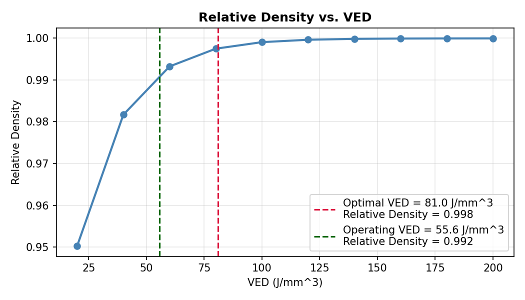
Distribution Fit Validation
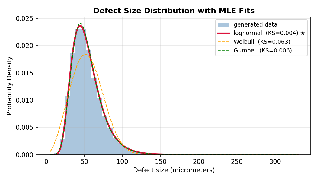
Three candidate distributions were fit to the synthetic defect population by maximum-likelihood estimation (MLE) and ranked by the Kolmogorov–Smirnov (KS) statistic. The best fit is selected by the lowest KS statistic.
Why lognormal?
Defect growth results from multiple multiplicative manufacturing effects— powder size variation, melt-pool instability, lack-of-fusion events, and gas entrapment—whose combined action produces a lognormal distribution in the limit. The lognormal distribution is the natural choice because it: guarantees positive defect sizes; reproduces the right-skewed distributions commonly observed in XCT measurements; naturally accommodates rare large defects; and is straightforward to sample in Monte Carlo simulations.
| Distribution | KS Statistic | p-value | Verdict |
|---|---|---|---|
| Lognormal ★ | 0.0064 | 0.4643 | Best fit — selected |
| Gumbel | 0.0072 | 0.3243 | Intermediate |
| Weibull | 0.0656 | ≈ 0 | Substantially worse — rejected |
Fitted lognormal parameters: μln = −9.904, σln = 0.3579. The lognormal is selected as the best fit and used to represent the synthetic defect population throughout the workflow.
KS statistic: quantifies the maximum distance between the empirical distribution function of the sample and the cumulative distribution function of the reference distribution. A lower KS statistic indicates a better fit; a high p-value means the observed distance is consistent with random sampling from that distribution.
Reliability Analysis
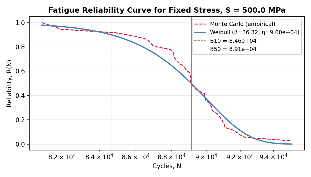
The reliability, R(N), is the fraction of specimens surviving beyond N cycles:
A two-parameter Weibull model is fitted for comparison with empirical survival curves:
where η is the characteristic life (R = e−1 ≈ 36.8% survival) and β is the shape parameter. A large β indicates a tight fatigue-life distribution; a small β indicates high scatter.
The large β value (≈ 36) indicates a very narrow fatigue-life distribution in the synthetic dataset. This is expected: all synthetic specimens were generated under identical process parameters, so the only source of scatter is defect-size variability. In a real experimental dataset, additional scatter from microstructure, surface condition, and residual stress would substantially reduce β, typically to values in the range of 2–5 for AM fatigue data.
PSN Sensitivity & Variability Curves
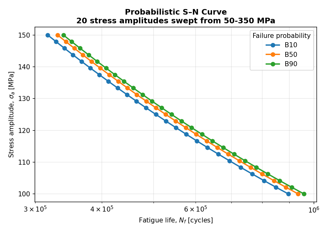
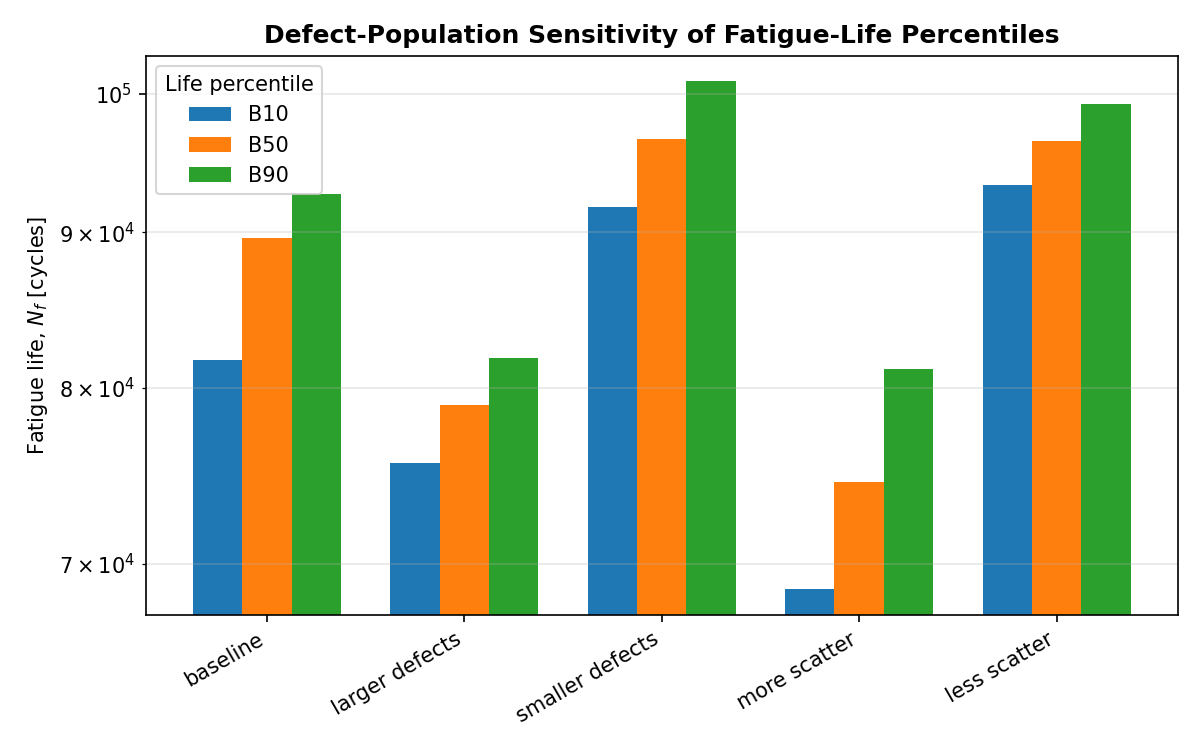
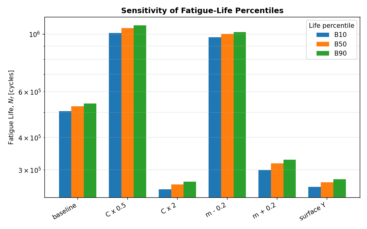
Sensitivity studies were performed by varying each Paris-law and defect-population parameter independently while holding all others fixed, and observing the shift in B10, B50, and B90 fatigue lives. The key observation across all studies: parameters affect the mean life much more than the variability. This separates two distinct phenomena: variability is controlled by defect population statistics, and sensitivity is controlled by Paris-law parameters.
Very influential: C × 0.5 roughly doubles fatigue life; C × 2 roughly halves it. Life is inversely proportional to C, consistent with the analytical solution Nf ∝ 1/C. A factor-of-two uncertainty in C produces an approximately factor-of-two change in predicted life.
The most sensitive parameter. A change of ±0.2 in m changes life by roughly a factor of 4–5. This is expected because m appears in multiple places in the fatigue-life equation — in the defect-size exponent (1 − m/2) and in the stress-range exponent (−m) — amplifying changes nonlinearly.
Surface defects reduce life relative to internal defects. Increasing Y from 0.50 to 0.65 increases ΔK, accelerating crack growth and reducing fatigue life. This is consistent with experimental observations that surface and subsurface defects are the most detrimental initiation sites.
Larger defects reduce life, as expected from Nf ∝ a01−m/2. Larger initial defects produce larger ΔKi, faster crack growth, and shorter life. Conversely, smaller defects (the goal of manufacturing optimization) extend life. This is the manufacturing-to-reliability connection the framework is designed to quantify.
Scatter has almost the same effect as mean defect size on B50: more scatter shifts B50 from 89K to 75K cycles; less scatter shifts it to 96K. This is because fatigue is controlled by the largest defect: when scatter increases, more extreme defects appear, maximum defect sizes grow, and fatigue life decreases. This is an extreme-value statistics result.
B10, B50, and B90 move together across all parameter variations. The spacing between them barely changes. So parameter variations shift the entire life distribution without substantially widening it. B90 moves more than B10 when defect scatter increases, meaning greater scatter mainly shifts the distribution rather than drastically widening it.
Model A vs. Model C: Feature Depth Comparison
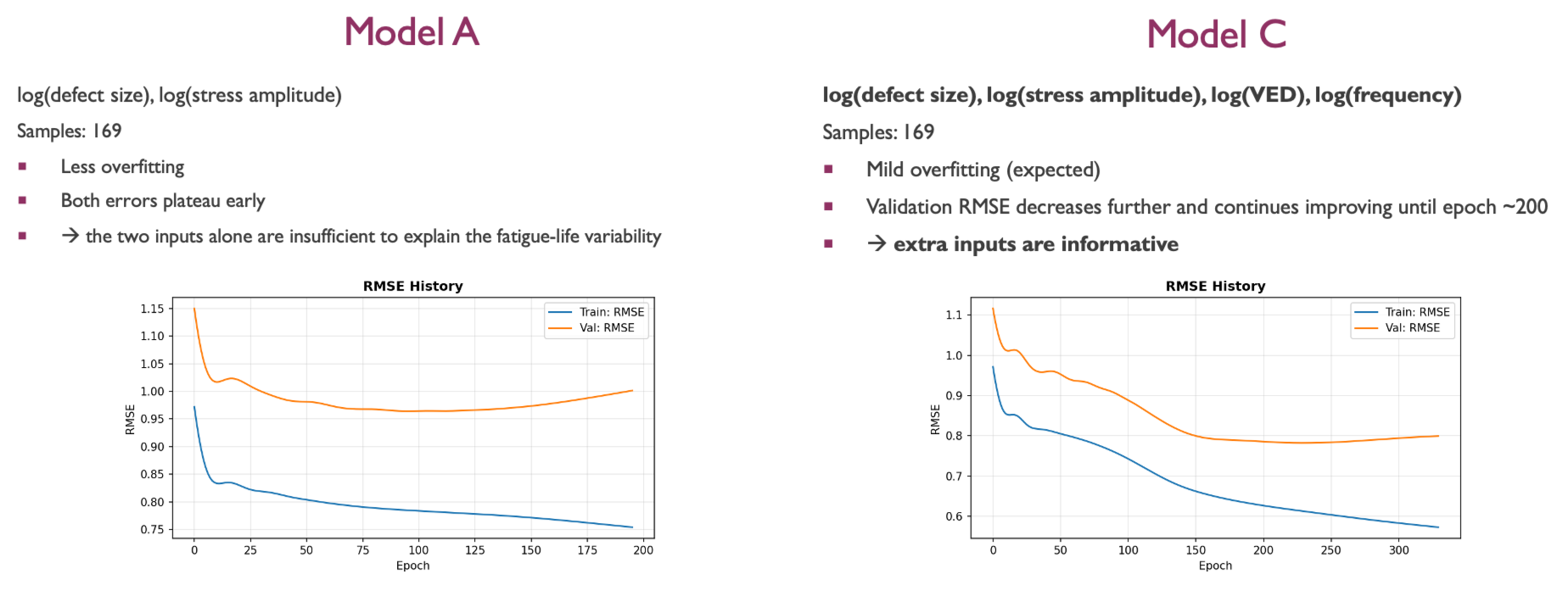
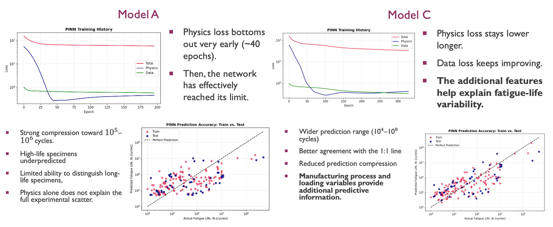
The clearest demonstration of what feature depth buys comes from comparing Model A (physics-only inputs) against Model C (physics + manufacturing process + loading frequency). Both are trained on 169 samples from the Zhang and Xu (2023) database with the same PINN architecture and loss weighting.
Why does adding VED and frequency help?
Defect size and stress amplitude are the primary drivers of fatigue life in Paris-law theory, and Model A reflects exactly that. However, experimental scatter in AM fatigue is caused by more than just defect size: the manufacturing process determines not just how many defects exist, but their morphology, spatial distribution, and surface proximity. Loading frequency affects crack-tip plasticity and environment-assisted cracking. Model A cannot distinguish between two specimens with the same defect size and stress but different manufacturing histories or test frequencies. Model C can.
The physics loss behavior is the clearest diagnostic: in Model A, the physics loss bottoms out at ~40 epochs and stops moving, indicating the network has learned everything the two inputs can teach it and is already constrained by the Paris-law residual. In Model C, the physics loss continues decreasing alongside the data loss well past 40 epochs — meaning the additional features are genuinely reducing the gap between the model and physical reality, not just fitting noise.
Key takeaway: Physics-informed inputs (defect size, stress) are necessary to ensure the model respects crack-growth mechanics. But the manufacturing and loading context are necessary to explain the scatter that pure fracture mechanics cannot account for. The best model combines both, which is exactly the case for physics-informed ML applied to AM fatigue.