AI Approaches for Fatigue-Life Prediction in Additive Manufacturing
A physics-informed neural network (PINN) to predict fatigue life in AM materials with minimal data.
Summary
Laser powder bed fusion (L-PBF) can produce complex metallic parts with high design flexibility, but process-induced defects—lack-of-fusion pores, keyhole porosity, surface roughness—make fatigue-life prediction extremely difficult. Two specimens produced under identical conditions can fail after very different numbers of cycles, because fatigue is controlled by stochastic defect populations and the physics of crack growth.
This project developed a computational workflow linking L-PBF process parameters to fatigue-life distributions through fracture mechanics and physics-informed machine learning. The goal was not to produce a black-box predictor, but a physically constrained model that remains consistent with known crack-growth theory even on sparse, noisy industrial datasets.
This project was done as a research internship with Institut de Mécanique et d’Ingénierie (I2M) in Bordeaux, within the Arts et Métiers research environment, in collaboration with CETIM.
This is only a fraction of the project. To see the full progress report in the form of a PowerPoint, click here.
Skills demonstrated: Physics-informed neural networks (PINNs), Paris–Erdogan crack-growth modeling, Shiozawa normalization, Monte Carlo simulation, extreme-value statistics (GEV), Weibull reliability analysis, feature engineering, train/test split design, loss-weight sensitivity analysis, data cleaning and unit harmonization
Tools & Libraries: Python, PyTorch, NumPy, pandas, scikit-learn, Matplotlib, SciPy, Torch, Git/GitHub
Data: Synthetic (Monte Carlo), Zhou et al. (2025) experimental dataset (n = 30), Zhang and Xu (2023) AM fatigue database (n > 500)
Key Finding
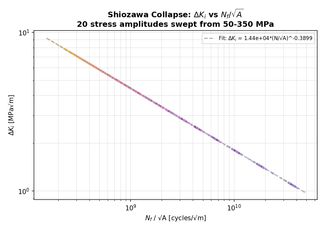
The Shiozawa normalization collapse reproduced the theoretical slope of −1/m = −0.3899 exactly to four decimal places across 20 stress amplitudes, thus confirming the full pipeline from process parameters through defect statistics to fatigue life is physically consistent.
Links
Introduction
Fatigue testing is expensive and slow, and AM fatigue datasets are typically sparse. At the same time, the relevant physics—Paris-law crack growth, Murakami defect-size effects, geometry correction factors—is only partially captured by standard data-driven models. A useful model must respect the known fracture-mechanics relationship between defect size, stress range, and fatigue crack growth, while still learning from experimental scatter.
Rather than treating the physics as a separate analysis, a physics-informed neural network (PINN) embeds a Paris-law residual directly into the loss function, penalizing predictions that are inconsistent with crack-growth theory. The physics term acts as a regularizer, especially valuable when data is scarce and overfitting is a big risk.
Overall Workflow
The project developed two parallel workflows. The synthetic branch built and verified the probabilistic fracture-mechanics framework from first principles. The experimental branch adapted the methodology to real literature fatigue data and PINN training. Overall, eleven models, four of which were ANNs to compare with the PINNs of the same data, were built across seven datasets and three materials. To view all of these models, please take a look at the final progress report.
Synthetic Branch
① Process Parameters → Volumetric Energy Density (VED)
Laser power, scan speed, hatch spacing, and layer thickness are combined into VED = P / (v h t).
② VED → Defect Density & Defect Population
A quadratic empirical model maps VED to defect density. Defect sizes are drawn from a lognormal distribution; defect counts per specimen follow a Poisson model.
③ Maximum Defect Extraction (GEV)
Because fatigue failure is governed by the largest defect present, only the maximum Murakami √A parameter per specimen is retained. The distribution of maxima is fitted with a Generalized Extreme Value (GEV) model.
④ Paris-Law Fatigue Life
Closed-form integration of the Paris–Erdogan law yields Nf from the initial defect size, applied stress range, and geometry correction factor Y.
⑤ Reliability & Shiozawa Validation
Weibull fits generate B10/B50 reliability curves. Shiozawa normalization provides a model-independent check: if the feature engineering is correct, data at all stress levels should collapse onto a single log-log line of slope −1/m.
Experimental Branch
① Data Cleaning & Feature Engineering
The Zhou et al. (2025) Ti-6Al-4V dataset (n = 30) and the Zhang and Xu (2023) AM fatigue database were cleaned, unit-harmonized, and reformatted. Four model variants (Models A–D) were constructed with progressively deeper input features.
② Defect Position Classification & Geometry Factor Assignment
Defects within 200 µm of the surface are classified as surface/subsurface (Y = 0.65); deeper defects are internal (Y = 0.50). This threshold follows Zhou et al. (2025).
③ Paris-Law Baseline Calculation
An analytical Nf is calculated for each sample. This becomes the physics target inside the PINN loss, so the network is penalized when predictions deviate from it, without being forced to match it exactly.
④ PINN Training & Evaluation
A two-hidden-layer PyTorch network with tanh activations is trained with a combined data + physics loss. Loss weighting (λdata, λphysics) is the primary tuning challenge. A grid search confirmed the Liao et al. (2025) weighting scheme (λdata = 100, λphysics = 1) provides the best balance.
Synthetic Dataset Generation
Before applying any machine learning to experimental data, a fully synthetic fatigue dataset was generated from first principles. This served two purposes: it allowed the probabilistic framework to be built and tested end-to-end before real data were introduced, and it provided a controlled validation environment.
Step 1: Defect Density from VED
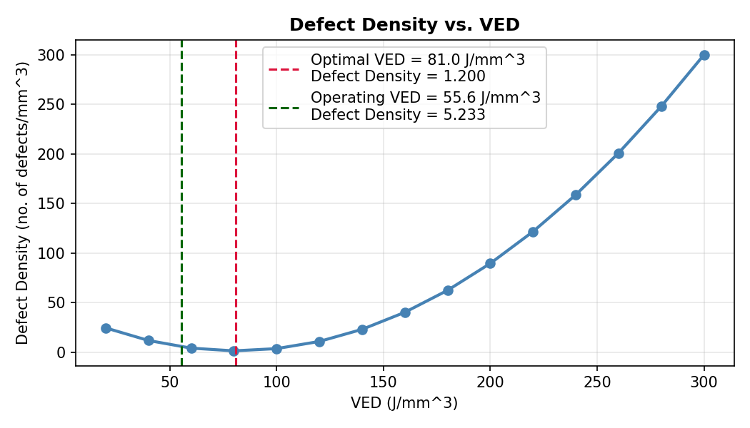
Defect density is modeled with a quadratic empirical relationship centered on the optimal VED:
ρd(VED) = α (VED − VEDopt)² + ρd,opt
where ρd,opt = 1.2 defects/mm³ (minimum at VEDopt) and ρmax = 300 defects/mm³ at VEDmax = 300 J/mm³.
The parabolic form captures the physical observation that both under-melting (lack-of-fusion pores) and over-melting (keyhole porosity) increase defect density. At the operating VED of 55.56 J/mm³, calculated from the literature process parameters, the model predicts ρd ≈ 5.23 defects/mm³.
Step 2: Synthetic Defect Population
Defect sizes are drawn from a lognormal distribution, physically motivated by the multiplicative nature of pore formation (powder size variation, melt-pool instability, lack-of-fusion events, gas entrapment). The number of defects per specimen is drawn from a Poisson distribution with an expected count λ = ρd · Vgauge, where Vgauge ≈ 196 mm³ is the assumed cylindrical gauge volume. This Poisson model naturally introduces specimen-to-specimen variability, even under identical process parameters—some specimens contain fewer defects than average, others more—propagating directly into fatigue-life scatter.
Three candidate distributions were fitted to the synthetic defect population by maximum-likelihood estimation and ranked by the KS statistic. The lognormal provided the best fit (KS = 0.0064, p = 0.4643), with fitted parameters μln = -9.904, σln = 0.358. Full distribution fit results are in the Appendix.
Step 3: Critical Defect and Generalized Extreme Value (GEV) Model
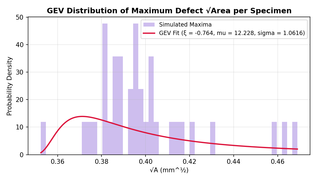
Fatigue failure is governed primarily by the largest defect present in a specimen. From each simulated specimen, only the maximum Murakami parameter √A is retained. This is the critical transition from manufacturing statistics to fatigue modeling: rather than tracking thousands of individual pores, the framework identifies the single defect most likely to control crack initiation.
The resulting distribution of maximum defect sizes across all specimens is fitted with a Generalized Extreme Value (GEV) distribution, with parameters estimated by MLE:
F(x; ξ, μ, σ) = exp{ −[1 + ξ((x − μ)/σ)]−1/ξ }
Fitted parameters: shape ξ = −0.761, location μ = 12.219, scale σ = 1.044. The negative shape parameter (ξ < 0) indicates a Weibull-type GEV, with a finite upper bound on the maximum defect size, which is physically sensible for a bounded manufacturing process. The GEV fit was confirmed as adequate across the simulated population.
Step 4: Fatigue Life and Reliability
Using the maximum defect from each specimen as a_i, the closed-form Paris-law equation yields a distribution of fatigue lives across the synthetic population. This distribution is then fitted with a two-parameter Weibull model to generate B10/B50/B90 reliability curves, which provide a full probability-of-survival curve as a function of cycles. The Weibull shape parameter β ≈ 36 in the synthetic case reflects very tight scatter, expected because the only source of variability is defect size under identical process conditions. Full reliability results are in the Appendix.
Key Equations
Paris–Erdogan Crack-Growth Law
where a is crack size, N is number of cycles, C and m are material constants, and ΔK is the stress-intensity factor range. For L-PBF Ti-6Al-4V: C = 7.69 × 10⁻¹¹, m = 2.565 (Wang et al., 2022).
Closed-Form Fatigue Life
Derived by integrating the Paris law from initial defect size ai to final crack size, assuming af ≫ ai (Shimatani et al., 2010). Y = 0.65 for surface defects, Y = 0.50 for internal defects.
PINN Loss Function
The data loss fits experimental fatigue lives; the physics loss penalizes deviations from the analytical Paris-law prediction. When λphysics is too large, the network collapses toward the analytical curve and underpredicts long-life specimens. When too small, the PINN becomes a standard neural network.
Results & Discussion
Physics Validation: Shiozawa Collapse
The Shiozawa normalization is a model-independent physics check on the synthetic data generated. If the feature engineering—defect-size extraction, stress-range conversion, geometry-factor assignment—is correct, data from specimens with different defect sizes and stress levels should all collapse onto a single log-log line with a slope of -1/m.
When swept across 20 stress amplitudes from 50–350 MPa, the fitted slope is -0.3899, matching the theoretical prediction of -1/m = -0.3899 exactly to four decimal places. The slope comes directly from the Paris constants and the defect statistics, with no tuning.
PINN Verification on Synthetic Data
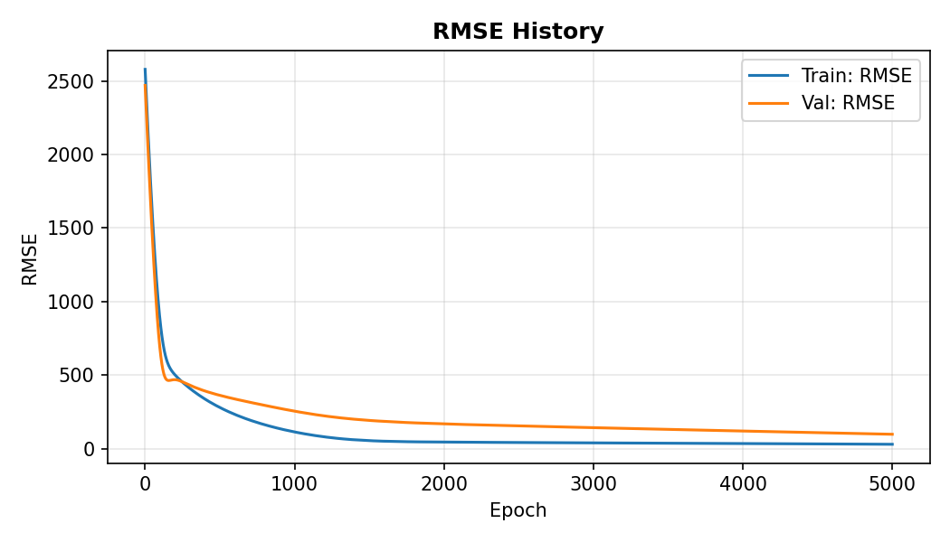
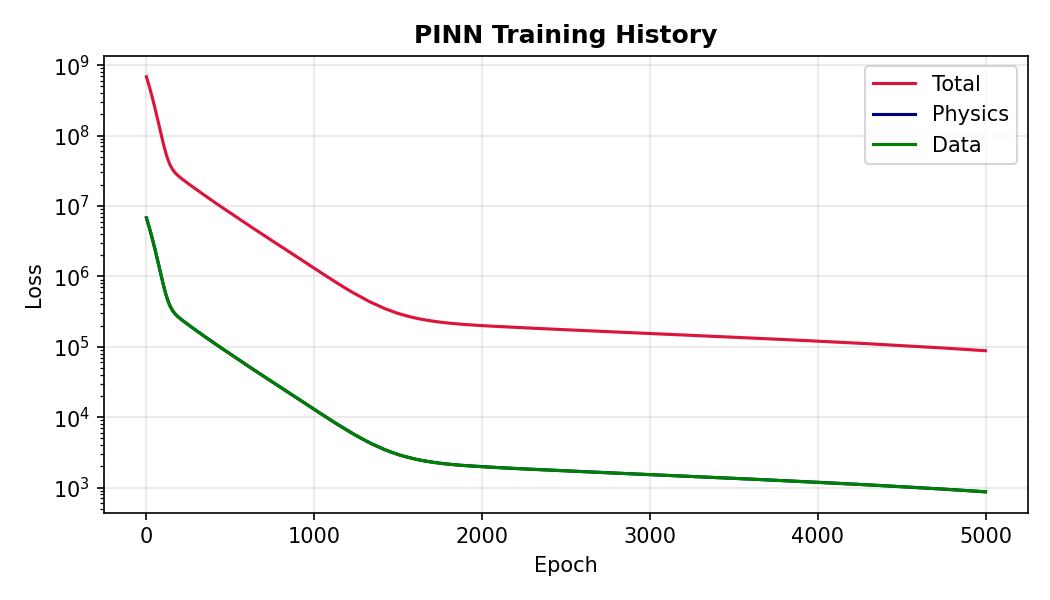
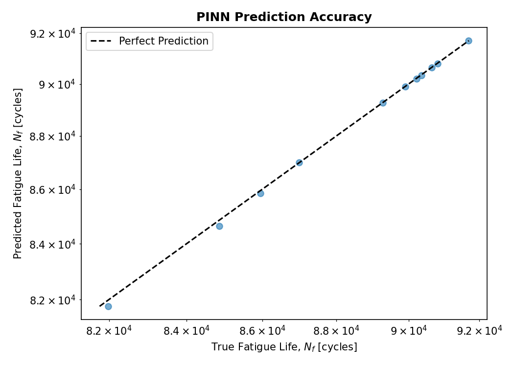
Before applying the PINN to experimental data, the model was trained on the synthetic dataset. Because the synthetic fatigue lives and the physics loss are derived from the same Paris-law relationship, this stage is a verification of the implementation rather than a predictive test. The network converged smoothly after reducing the Adam learning rate from 10^-3 to 10^-4. Training and validation RMSE remained nearly identical with no evidence of overfitting, and predicted vs. actual fatigue lives showed near-perfect agreement, thus confirming the architecture, scaling procedures, and loss formulation were implemented correctly.
PINN on Experimental Data
Zhou et al. (2025)
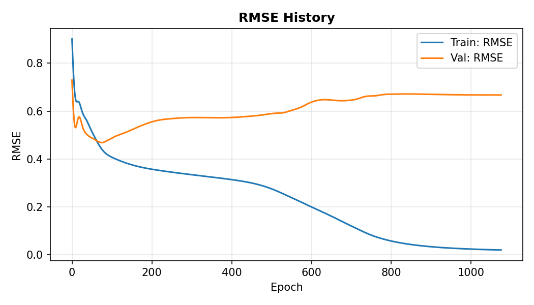
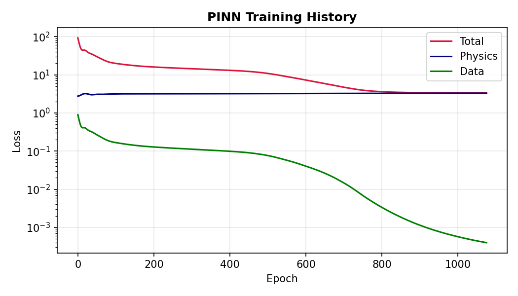
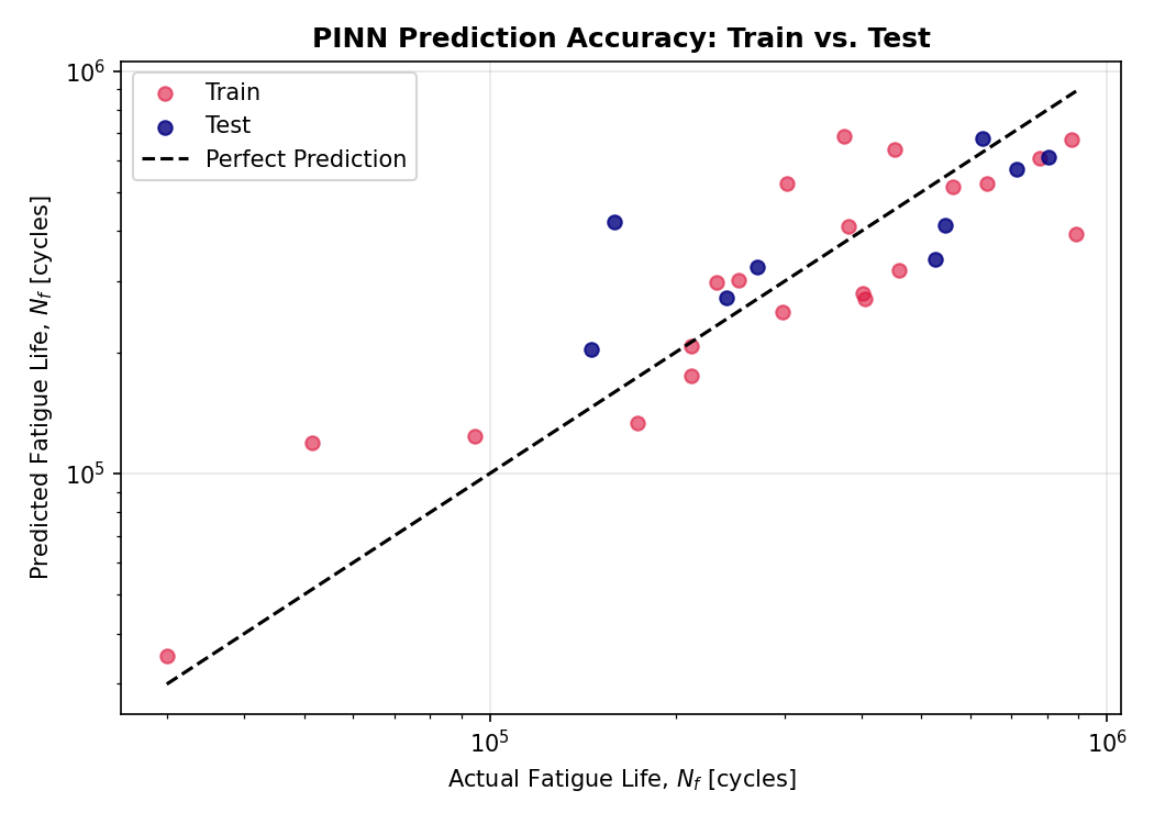
Applied to the 30-sample Zhou Ti-6Al-4V dataset (21 train / 9 test), the PINN faced a fundamental challenge: the analytical Paris-law model systematically underpredicts long-life specimens, because the simplified formulation omits crack-initiation effects, threshold behavior, residual stresses, and microstructural variability. As a result, the physics loss remained nearly constant during training while the data loss decreased to ~10^-3, indicating the network was fitting the experimental data while making little progress toward reducing the Paris-law residual.
The predicted vs. actual plot shows regression-to-the-mean behavior: low-life specimens are overpredicted, high-life specimens are underpredicted. The validation RMSE reaches a minimum around 50–100 epochs before increasing to ~0.64, while training RMSE continues decreasing to ~0.05—a classic sign of overfitting on a 21-sample training set.
Zhang and Xu (2023) Database
The Zhou dataset is too small to fully evaluate the PINN. A substantially larger fatigue database from Zhang and Xu (2023), containing AM fatigue data across multiple materials, loading conditions, and defect descriptors, was cleaned, standardized (units and column names were homogenized), and integrated into the framework. The database is filtered for a consistent Ti-6Al-4V, L-PBF subset with R = 0.1, fatigue temperature = 25°C, environment = “air”, build direction = 90°.
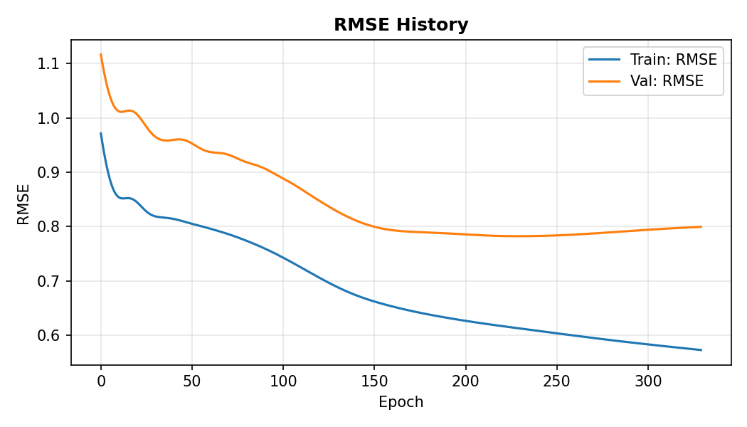
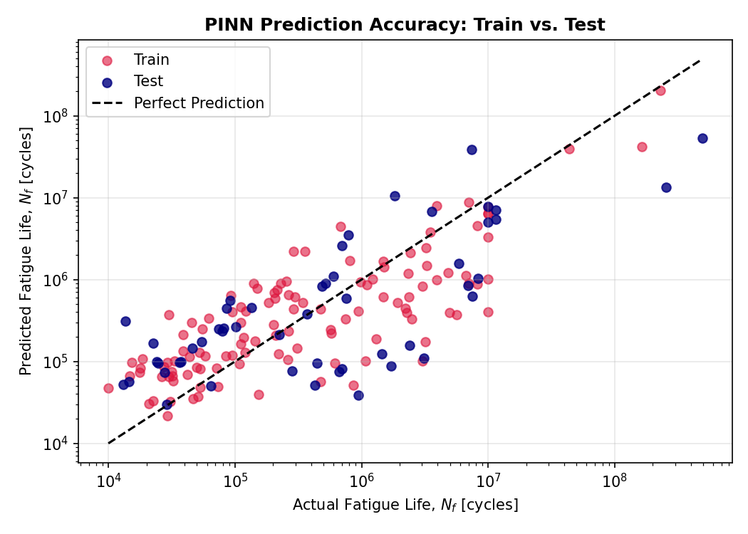
The PINN uses Model C, as it showed improvement over the other models, and takes log(defect size), log(stress amplitude), log(VED), log(frequency) as the inputs and log(fatigue life) as the output. The prediction range widens from the compressed Zhou behavior (10^5-10^6 cycles) to the full experimental span (10^4-10^8 cycles), and agreement with the 1:1 line improves substantially.
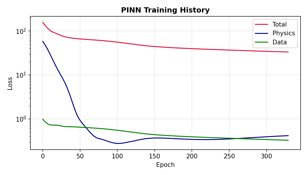
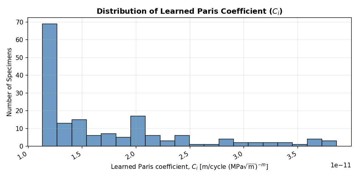
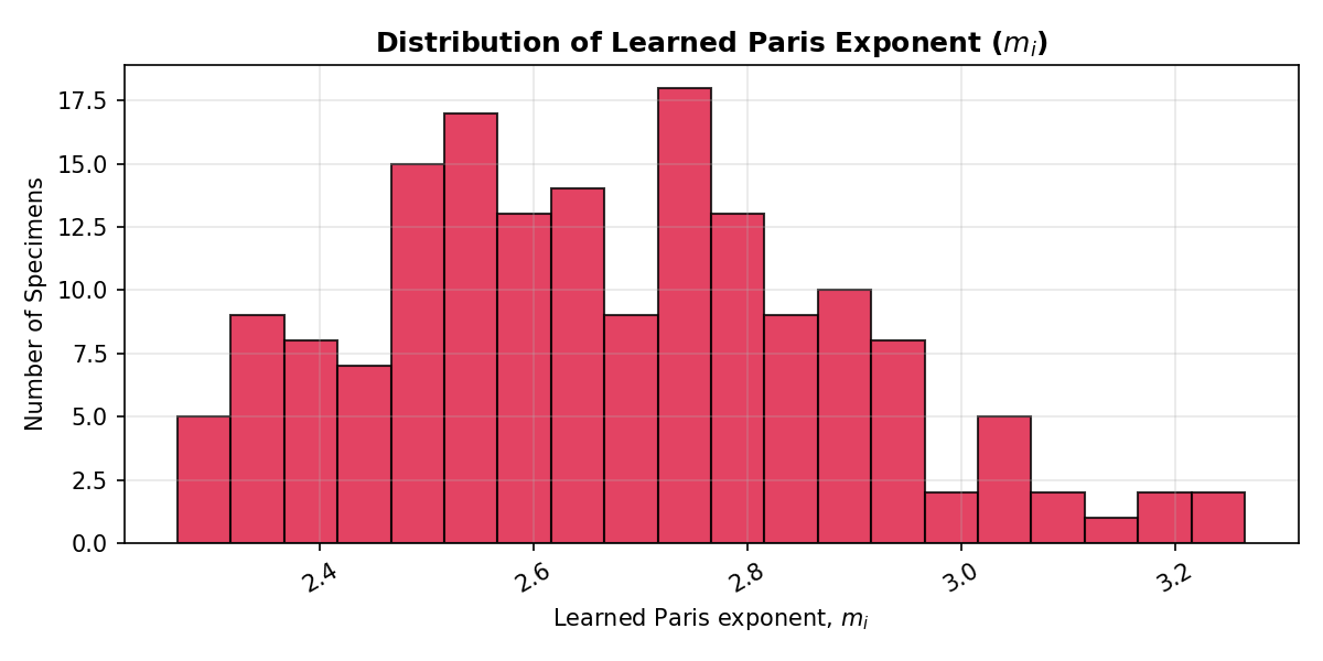
The Paris constants, C and m, are treated as trainable parameters. This allows the model to better fit the physics loss, as seen in the training history plot.
Feature Engineering: Four Model Variants
To test what actually drives fatigue-life scatter in the Zhang and Xu (2023) database, four model variants were constructed with progressively deeper input features. Adding inputs also reduces usable samples since missing values are dropped, so each variant represents a deliberate data-vs-features trade-off. To compare models, the same 169 samples found in Model C are used in Models A-C. For a complete comparison between Models A and C, see the Appendix.
| Model | Inputs | Samples | Key observation |
|---|---|---|---|
| A | log(defect size), log(stress amplitude) | 169 | Physics-only baseline. Less overfitting, but both losses plateau early, so the two inputs alone cannot explain fatigue-life variability. |
| B | A + log(VED) | 169 | Adding manufacturing process context. |
| C | A + log(VED) + log(frequency) | 169 | Physics loss stays lower longer; data loss keeps improving. Extra inputs are informative. Wider prediction range, better 1:1 agreement, reduced compression. |
| D | C + Kt, E, yield strength, UTS, elongation | <169 | Full material/mechanical features. Young's modulus alone has >10,000 missing values in the database, so adding it costs significant data. |
Trainable Paris Parameters
The latest version of the PINN (results shown) allows the Paris constants, C and m, to be learned during training rather than fixed to literature values. This follows the approach of Liao et al. (2025) and enables the model to adapt the physics baseline to the specific material system and dataset, rather than relying on published values that may not perfectly match experimental conditions.
The model learns 𝐶 to be between 1.13×10⁻¹¹ and 3.86×10⁻¹¹ with an average of 1.72×10⁻¹¹. The value of 𝑚 is learned to be between 2.27 and 3.27 with an average of 2.67.
The initial values from literature were C = 7.6899×10⁻¹¹ (m∕cycle)/(MPa√m)^m and m = 2.56 from Wang et al. (2022). Comparing the literature values with the learned parameters, the learned parameters, and thus the model, remain physically realistic while improving fatigue-life prediction.
Data Availability Study
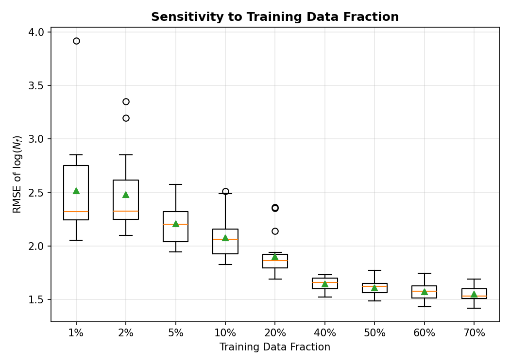
The model was retrained on 1–70% of the database across 20 random train/test splits per fraction to understand the minimum data required for a reliable prediction. Error decreases substantially with the first 5–20% of data (approximately 8–33 samples). Beyond 20%, additional data provides diminishing improvements in performance, suggesting that most of the benefit of the large database is captured with a modest training subset.
Lessons Learned & Limitations
The most important insight from the experimental branch is that the primary limitation is not the PINN architecture, but rather, it is the mismatch between the simplified Paris-law baseline and the experimental fatigue lives. Real fatigue behavior includes crack-initiation phases, threshold ΔK effects, and microstructural variability that are not captured by the closed-form Paris-law formulation. The physics loss cannot be meaningfully reduced during training because the analytical model systematically underpredicts long-life specimens.
This is not a failure of the methodology. Rather, the PINN framework exposed the limitations of the underlying physics assumption in a way that a pure data-driven model would not, because the physics residual makes the gap between model and data explicit and measurable. Improving the physics constraint(crack-initiation terms, threshold effects, updated C and m estimation) is the most productive next direction.
The synthetic framework demonstrated that the underlying fracture mechanics are implemented correctly: the Shiozawa normalization reproduced the theoretical slope exactly, and the Weibull reliability analysis produced physically reasonable B10/B50 lives with a large shape parameter (β ≈ 36), discussed in the Appendix, reflecting the narrow scatter expected when only defect-size variability is present.
Conclusions & Next Steps
A probabilistic fatigue-life prediction framework was successfully developed, linking L-PBF process parameters to fatigue-life distributions through defect statistics, fracture mechanics, and physics-informed machine learning. The framework integrates defect generation, extreme-value analysis, Paris-law calculations, Shiozawa normalization, reliability analysis, and PINN training within a single traceable computational pipeline.
Recommended next steps include: completing PINN training on the full Zhang and Xu (2023) database; systematic comparison of the analytical baseline, a data-only neural network, and the PINN; incorporating crack-initiation and threshold effects into the physics constraint; and adding uncertainty quantification for engineering design applications.
References
Liao et al. (2025). A physics-informed neural network method for identifying parameters and predicting remaining life of fatigue crack growth. International Journal of Fatigue, 191:108678.
Murakami, Y. (2019). Metal Fatigue: Effects of Small Defects and Nonmetallic Inclusions. Academic Press.
Paris, P. and Erdogan, F. (1963). A critical analysis of crack propagation laws. Journal of Basic Engineering, 85(4):528–533.
Shimatani et al. (2010). Effect of surface residual stress and inclusion size on fatigue failure mode. Procedia Engineering, 2:873–882.
Wang et al. (2022). Fatigue performance at ultra-low porosity of Ti6Al4V produced by L-PBF. SSRN Electronic Journal.
Zhang, Z. and Xu, Z. (2023). Fatigue database of additively manufactured alloys. Scientific Data, 10:249.
Zhou et al. (2025). A general physics-informed neural network framework for fatigue life prediction. Engineering Fracture Mechanics, 322:111136.